I was talking to one of my professors about mathematics after class one day this semester and he told me about an interesting math question that had occurred to him while doing algebra with one of his kids. They had been looking at the equation for the top half of a circle: , which looks like this if you graph it:

Unlike the graphs of many simple functions, like or , which are defined for almost all real numbers, this function is only defined between -1 and +1. This is because if is less than -1 or greater than +1, is greater than 1 and thus is negative. Since the square root of a negative number is an imaginary number, these solutions to the equation do not appear on this simple 2D x and y plot. But that’s not to say these solutions don’t exist.
This led my professor to ask the question: Well what do these solutions look like? What happens to the graph of if you allow to be imaginary? It seems a fairly simple question, but it wasn’t obvious what that answer was. We tried to make a rough estimate on the chalkboard, but we both wanted a computer visualization.
When I had some spare time, I started working on a simple program to graph the extension of simple x and y equations into the complex plane. These objects are technically four dimensional (the four axes are real x, imaginary x, real y, and imaginary y), so I knew I couldn’t graph the whole shape all at once. But I could graph a series of 3D “slices” which, taken together, would represent the 4D object: just as you can represent a 3D object in 2D by taking a series of 2D cross sections, you can represent a 4D object in 3D by taking a series of 3D cross sections. But I fairly quickly ran into some issues with this plan, the first being how to concretely define this 4D object. I wanted to graph the full circle, not just the top half, and the equation for that in real x and y is simply . In order to graph this in two dimensions on a computer, what one can do is graph the boundary of the solid area , for instance using the Marching Squares algorithm. But this doesn’t obviously extend into the complex plane, because the operation does not have an obvious extension to complex numbers.
I came up with two modified definitions of a circle in two dimensions to solve this problem: and . Both of these definitions can be extended to complex numbers, because the absolute value operation has an obvious equivalent for complex numbers: taking the magnitude of the number.
Having defined these 4D solids, I was able to make a program to graph 3D slices of them. I used the THREE.js library to handle the complexities of 3D rendering (WebGL, lighting, controls, etc.), leaving me to actually generate a triangle mesh approximating the 3D slice. To do this, I reused some Marching Cubes example code for THREE.js. The Marching Cubes algorithm is the 3D analog of the Marching Squares algorithm. It takes in a 3D scalar field (a function which takes in a coordinate in 3D space and returns a scalar number) and produces a triangle mesh approximating boundary of the solid volume where the field value is less than 0. (i.e., the surface where the field value transitions from negative to positive).
To convert my 4D solid into a scalar field like this, I just needed to do a little rearrangement of the formula. For example, becomes the 4D scalar field (for complex x and y, of course). The parts of this field where are exactly where . Converting into this form posed some difficulty, since is never less than 0 and thus the Marching Cubes algorithm will render nothing. I solved this problem by instead graphing , where is some small (but non-zero) constant.
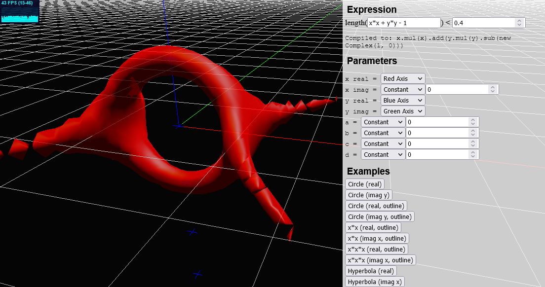
With all that settled, I was finally able to generate a visualization of extended to the complex plane:

Here’s what you’re looking at in the image above:
The formula being graphed is , with .
The red axis represents real x, the blue axis real y, and the green axis imaginary y
Thus, the regular 2D plane with real x and y is the plane defined by the red axis and the blue axis. If you took a cross section along this plane, you’d see something like this:
 which is what we expect for
.
which is what we expect for
.As we can now see from the 3D graph, this cross section does not include all of the solutions to the equation: there are four hyperbolic “arms” in a perpendicular plane. These arms in the real x, imaginary y plane are the additional solutions we were originally trying to visualize.
Now that I have this program working, it’s pretty easy to see what lots of other simple equations look like in the complex plane. Click on the link below and take a look!